Feb 19, 2026

Melody as a Log-Derivative: Why Songs Survive Key Changes

This is a compact intuition-first post. For deeper treatment, see references. Content generated via LLM collaboration — see authorship note.

Why Songs Survive Key Changes

You recognize “Twinkle Twinkle Little Star” whether it starts on C or F♯.

Not because the absolute notes stay the same. They do not. Move from C major to D major and every note shifts: C→D, G→A, A→B. Different note names, different frequencies, different piano keys.

What stays the same is the pattern of intervals. And those intervals are fundamentally frequency ratios, not raw Hz differences.

Intervals Are Ratios, Not Differences

Consider two jumps that are both “100 Hz apart”:

200 Hz → 300 Hz: ratio of 1.5. That is a perfect fifth — one of the most recognizable intervals in music.
2000 Hz → 2100 Hz: ratio of 1.05 (~84.5 cents). That is smaller than a semitone, still clearly audible, and much narrower than a fifth.

Same Hz gap, very different musical meaning. Musical pitch intervals track frequency ratio (equivalently, differences in log-frequency), not raw Hz spacing.

You can verify this quickly. Play C3 with G3, then C5 with G5. In equal temperament both are the same interval class (7 semitones; ratio $2^{7/12} \approx 1.498$ , close to $3:2$ ). The Hz gap changes a lot, but the interval category does not.

Enter the Logarithm

If pitch is ratio-based, we want coordinates where ratios are easy to work with. That is exactly what logarithms do. The key identity:

\log\!\left(\frac{a}{b}\right) = \log(a) - \log(b)

Ratios become differences. Take two notes, 220 Hz and 330 Hz, and compute their distance in log-space (base-2, so the result is in octaves):

\log_2(330) - \log_2(220) = 8.366 - 7.781 = 0.585 \text{ octaves}

Now double both frequencies — a completely different register:

\log_2(660) - \log_2(440) = 9.366 - 8.781 = 0.585 \text{ octaves}

Different frequencies, different log values, same difference.

Multiply by 12 to convert octaves to semitones: $0.585 \times 12 \approx 7.02$ semitones. That is a perfect fifth, whether you play it at 220 Hz or 4400 Hz.

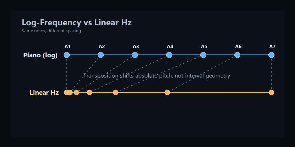
This means that on a log-frequency axis, equal ratios become equal distances. And that is exactly how a piano keyboard is built: in equal temperament, each key multiplies frequency by $2^{1/12} \approx 1.059$ . Equal key spacing = equal log-frequency steps = equal ratios.

Top: the piano spaces each octave evenly, while a linear Hz axis does not — low notes get crammed together. Bottom: the cochlea does the same thing. Each octave gets equal membrane length, even though the Hz range doubles each time (orange curve). This panel uses a simplified illustrative range, not a full hearing-range map.

The Ear Works in Log-Space

The cochlea — the spiral structure of the inner ear — is tonotopic: different positions respond best to different frequencies. High frequencies peak near the base; low frequencies peak near the apex. To first order, this place-to-frequency map is approximately logarithmic.

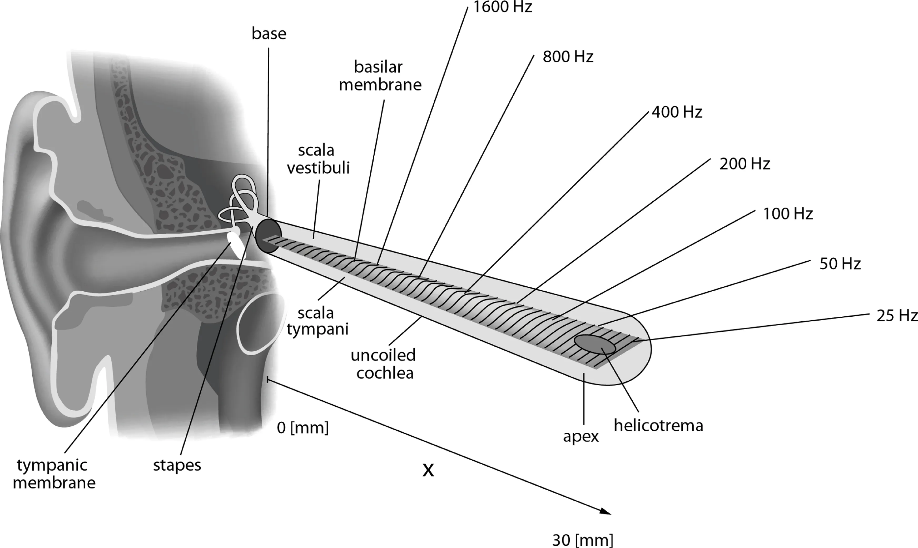
Uncoiled cochlea with basilar membrane, showing frequency regions from 1600 Hz at the base to 25 Hz at the apex

The cochlea, uncoiled. The basilar membrane widens from base (narrow, stiff, high-frequency) to apex (wide, more compliant, low-frequency). The labels suggest an approximately log-like map. In this schematic, the 25—1600 Hz labels are illustrative landmarks, not the full human audible range (~20—20,000 Hz). Diagram by Kern et al., CC BY 2.5.

Why this shape? The basilar membrane is narrow and stiff at the base, wide and compliant at the apex. A stiff region resonates at high frequencies (like a short, tight guitar string); a compliant region resonates at low frequencies (like a long, loose one). The stiffness drops roughly exponentially along the membrane’s length, which is the main driver of the logarithmic frequency map. Other factors — effective mass, damping, cochlear fluid coupling, active amplification by outer hair cells — refine the picture, but the stiffness gradient is the core of it.

Georg von Bekesy

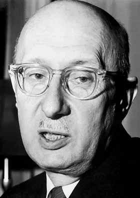
Georg von Bekesy worked this out in the 1940s—50s, earning the 1961 Nobel Prize in Physiology or Medicine. He dissected human cochleae, dusted the basilar membrane with silver flakes, and used strobe photography to watch it vibrate. What he saw was a traveling wave: sound entering the ear sends a ripple down the membrane, and the ripple peaks at a position determined by frequency. High-pitched sounds peak near the stiff base; low-pitched sounds travel further and peak near the compliant apex. Each point on the membrane is essentially tuned to a specific frequency — a physical frequency analyzer, with the frequency axis laid out approximately logarithmically.

The logarithm here is not just a convenient transform. The cochlea’s tonotopic map is a major reason interval perception aligns with ratios. Ratio detection is built into the hardware.

See It for Yourself

Now that we know intervals are ratios, and ratios become differences in log-space, here is the payoff. Change the key below and watch what happens:

Panel A: absolute frequencies shift with every key change.
Panel B: interval ratios between consecutive notes stay fixed.

Those ratios are the melody. The key change multiplies every frequency by the same constant, but the ratios — the log-differences — don’t budge.

Key:

Melody as a Derivative

Now we can state the key idea precisely.

In log-frequency space, a melody is a sequence of positions:

x_1, x_2, x_3, x_4, \ldots

The heard intervals are the differences between consecutive positions:

x_2 - x_1,\; x_3 - x_2,\; x_4 - x_3,\; \ldots

That is a discrete derivative of pitch in log-frequency coordinates.

Under key change (transposition), every frequency is multiplied by a constant $k$ , so each log-position gets $+\log(k)$ :

x_1 + \log(k),\; x_2 + \log(k),\; x_3 + \log(k),\; \ldots

Take differences again:

[x_2 + \log(k)] - [x_1 + \log(k)] = x_2 - x_1

The constant cancels. The interval sequence is unchanged. Melody, defined as the sequence of intervals in log-frequency space, is transposition-invariant.

Where It Breaks Down

This invariance is strong, but not absolute.

Timbre shifts with register. A melody in sub-bass and the same melody in mid-range can feel different because harmonic balance and auditory sensitivity change.
Extreme key changes. Push far enough and notes leave the range where pitch cues support melody robustly (roughly tens of Hz up to a few kHz).

These are limits on perception, not a contradiction of the core log-interval model. And the claim here is deliberately narrow: melody survives key changes because interval structure is preserved in log-frequency space. Questions about tonic, tonal gravity, and why one pitch feels like “home” are real and important, but they are a separate layer of perception.

References

Musical Consonance from Frequency Interactions — Companion post on psychoacoustic layers and why simple ratios tend to sound consonant.
The Physics Of Dissonance by Henry Reich (minutephysics) — Why simple frequency ratios sound consonant.
Dissonance: A Journey Through Musical Possibility Space by Aatish Bhatia — Interactive exploration of consonance through frequency ratios.
Georg von Bekesy — Wikipedia article on the physicist who discovered the traveling wave and mapped cochlear frequency response. Nobel Prize 1961.
Nobel Prize ceremony speech, 1961 — Presentation speech describing Bekesy’s discoveries.
Research Note: Melody as a Log-Derivative — Adversarial audit of the claims in this post, with primary sources and falsification criteria.

Authorship

I didn’t write any of this content. The text, visualizations, and interactive plots are the result of iterative collaboration and “LLM dueling” between Claude (Anthropic) and ChatGPT (OpenAI). The interactive component was implemented by Claude Code.